Introduction

Modern Styrofoam is an excellent building material for model builders. This material, which mostly comes as blocks or plates, can be excellently cut with a hot wire and almost any shape you can imagine and draw can be made from a block of Styrofoam using a CNC computer-controlled hot-wire foam cutting machine. In the market there are enough commercial CNC cutters. However, they have one common characteristic - namely, a fairly high price and thus are out of range of a normal mortal modeler. So the hobby community was looking for an inexpensive alternative that any interested modeler could master without essential technological effort. It should also meet the usual high accuracy requirements, the model builders usually have.

All styro-Cutters existing on the market work according to the portal principle. The cutting wire is moved by spindles parallel to the axes in a synchronized way or also independent of each other by steppers. You need precession spindles and this is the reason for the high price. For some time now, however, there are also solutions that have a precise mechanics and still have reasonable prices (for model builders).

H. Seybold has designed an ingenious CNC-controlled hot wire cutting machine using the cable winch setup and made it available to the public. This cutter can be built with very low resources. But you have to do it yourself, since no kits and no complete cutters are available at the moment. A further point has prevented a wide distribution: the very elaborate mathematics, which is necessary for an accurate control.

Both cutter types require a highly developed software for operation (Video). It has the task to guide the cutting wire and to allow accurate cuts. The present program ICE provides a basis to configure the cutting machine, to read cutting data, to store, to make appropriate representations and to perform the cutting process itself. In addition, ICE provides a cutter environment (CE) that goes far beyond the control of the cutting process. Meanwhile, this cost-free software has reached a level comparable to corresponding commercial products concerning quality and accuracy.

This manual applies to both cutter types. If there are deviations, it is explicitly pointed out. This manual is available as an online manual and always describes the current state of the software. ICE is basically a free software without any restrictions, which is freely available for downloading as a complete software package on the side of our model flying club MFC Rossendorf, which, like any other software, must be minimally configured before use. If ICE is operated on a portal cutter, the interface of Letmathe must be used, because no other interface is currently implemented.

Hot-wire cutting machine controllers are basically demanding time-critical applications. In order to achieve good cutting results, software and hardware components must be well coordinated. The environment required for ICE is explained in detail in the manual. Kludge is not supported by ICE!

This manual applies to both cutter types. If there are deviations, it is explicitly pointed out. The interested reader can learn about the theoretical basics of the CNC computer-controlled hot-wire foam cutting machine here.
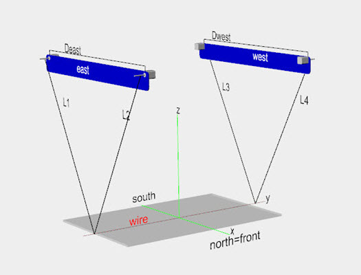
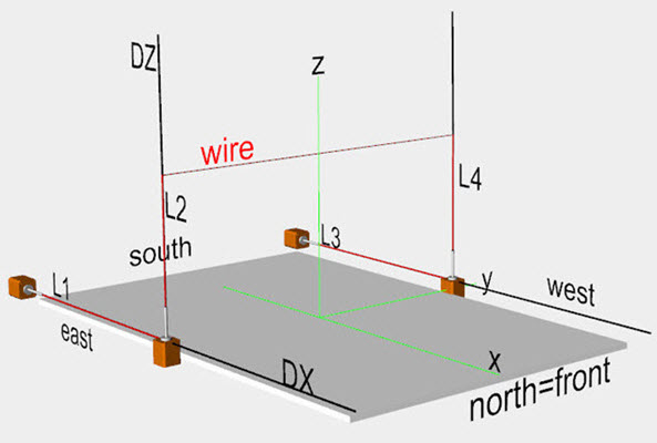
Requirements
To run the program, you must have some minimum requirements:
- You should have at least a moderately equipped PC with a parallel port. If it has none and that is certainly the case with modern computers, you can use very well the program, however, you cannot cut unless you let ICE communicate through a special USB connectivity with the cutter
- On the computer you should have administration rights; at least temporarily. The program was developed on a PC with Windows7,8,10 however, other operating systems should also work. Since this is a Java program, it also runs under Linux without any problems(but I have never published it!).
- On your PC you need to have installed a Java Runtime Environment as a prerequisite. If this is not the case, you can find instructions in chapter installation.
- Otherwise, unzip the downloaded file ICE.zip into a directory of your choice.
- If you want to cut, you should use the geometry data of your machine. It is also useful to read the tips!
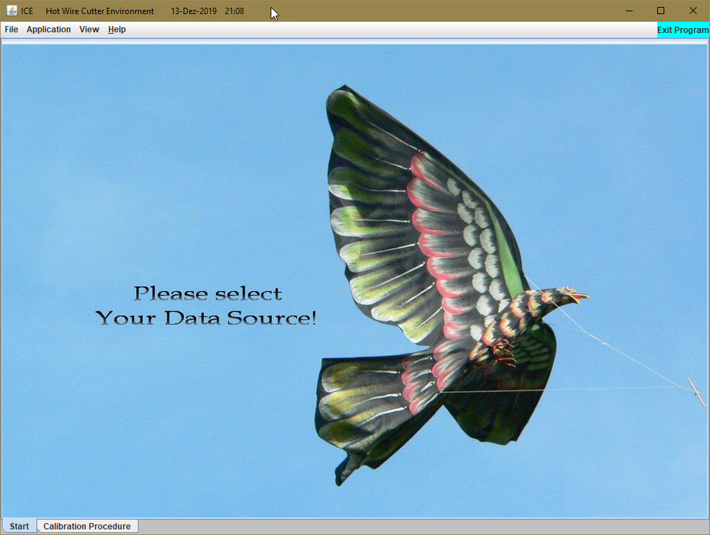
- Now start ICE.exe and the world should be beautiful ...
  To learn everything else you need to know, continue reading.

Data management

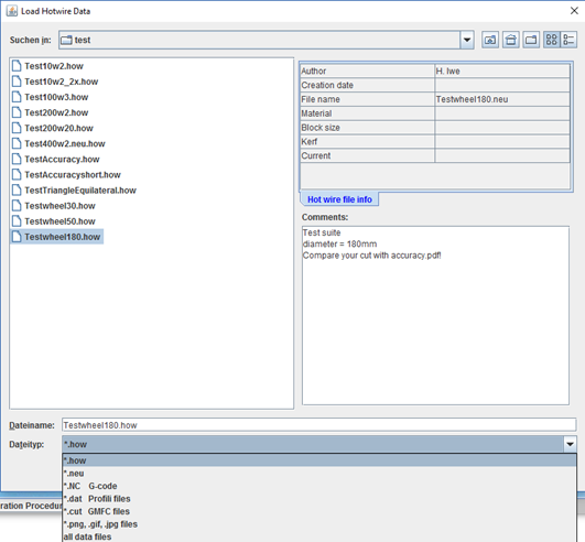
For cutting of objects made of foam, ICE requires CNC data. These are usually created with graphical or even better, with CAD programs (e. g. Profili). ICE provides an environment to read, manipulate and prepare such data for the cutting process. ICE is not a CAD program and will not do it in the future, although data can be generated to a limited extent for some recurring tasks. However, ICE provides tools by which the geometric figures can be further processed. At the present time, cutting data can be loaded via the following data formats.

*.nc or *.cnc (G-Code)
Unfortunately, G-code is not equal to G-code, but there are at least 83 bush dialects of them. In terms of model construction, it seems to me that the generation of 2D data with the help of BOcnc or Profili is very popular. Therefore I provided these two variants which differ significantly. Furthermore, I have extended the converter so that in the meantime a large intersection of NC codes is understood. Anyone who works with other formats should transform with Converter programs (smal support for this).
*.neu
This format was created by H. Seybold. It is derived from the G-code and was tailored and simplified to the needs of the cutting machine.
*.how
ICE uses a new data structure starting with the new version 1.2.0. Old data files * .new can only be read. Basically, the new data structure is used for saving.
*.dat
This format allows you to import airfoils.
*.cut
This format allows you to import GMFC-files.
*.png, *.gif, *.jpg
Images existing in these graphic formats can be loaded as master illustration for digitization/retracing by point-and-click.

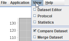
Using "View → Dataset Editor" you can inspect the read data in an own tab "Dataset Editor".

Save data (save)

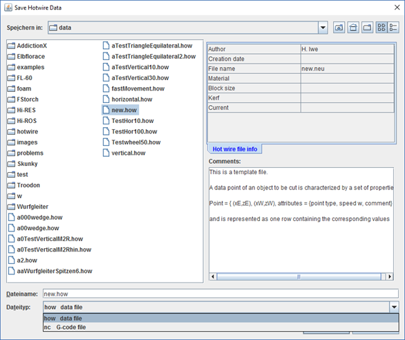
Data can be saved only if they previously have been loaded or generated by applications; otherwise the function save is not active. If data are available, they can be saved presently only in the format .neu or as G-code .nc. It does not matter whether the data were previously read or generated by applications. In any case, the data to be stored are always related to the graphic that appears in the tab "Diagram". Only the data whose graphic can be seen currently are stored. Besides, the origin of the data is irrelevant here.

ICE has a file information system. In the template you may fill in additional information if you want. On the one hand the standard text boxes are used to keep order, on the other hand, to collect information that you considered for some reason as important. All boxes are text fields, so you can write whatever you want, even entire novels! To inform the editor that you have written enough text, you must obligatory click into another field. Of course, you can edit the file with your favorite text editor, but please do not lay hands on the keywords.

Hotwire specific file:

Each time the program starts a Hotwire specific file is read:

hotwireGeometryData.prof

contains the properties of the cutting machine used

Data to set the Hotwire profile (.prof)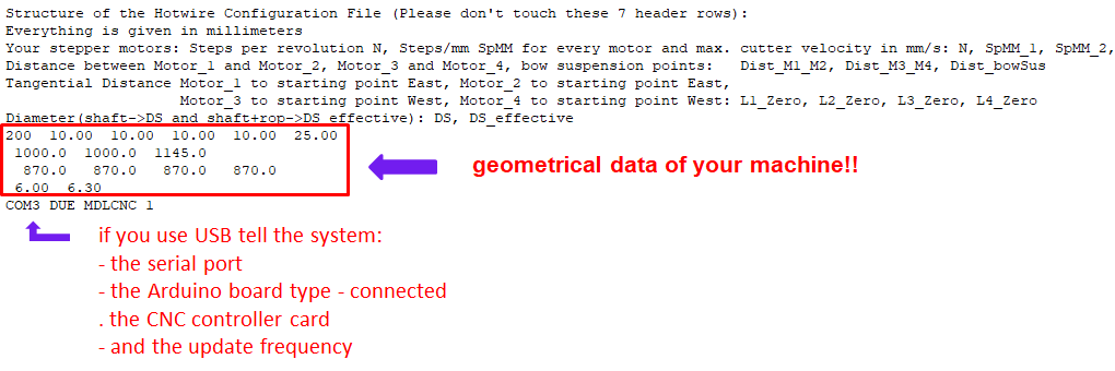

This file has the extension ".prof" and contains the above-mentioned variables as ASCII text. You can of course use your favorite editor to edit this file directly, and thus adapt to the needs of your own system. When editing please do not lay hands on the first 7 lines - they have to remain! Of course, in place of the numerical values given here, you have to insert the geometrical data of your machine! If you want to eliminate the radius correction, set for the effective radius simply zero, i.e. DS_effective=0.

If you use the USB interface you should inform your system which serial port is used by the Arduino Board and which type {NANO, UNO DUE} is connected (e.g. COM3 UNO). Otherwise let the line simply free. All of these basic parameters can be easily and comfortably adapted using the new Parameter Editor.

Instructions for checking your cutting machine you can get here.

Calibration
The Control Panel displays in the field Communication via whether the communication to the cutting machine can take place using the requested interface. The default is the parallel port. In the case that it was not found the value NO PARALLEL PORT appears. In this instance, of course, you cannot cut, but all other program functions are available.

After the start of the cutting machine, a calibration is absolutely required, i.e. the system must be brought in a defined position. The cutting wire has to be placed horizontally in the middle with a distance of z₀ above the xy plane. Sometimes during the cutting process, occasionally deviations are possible which require readjustments. If only the single controls of the step engines are available, a manual adjustment can be a very time consuming matter. For the experienced cutter this situation should not be a problem in comparison to the occasional cutter. For this reason, a module has been developed which simplifies this process.

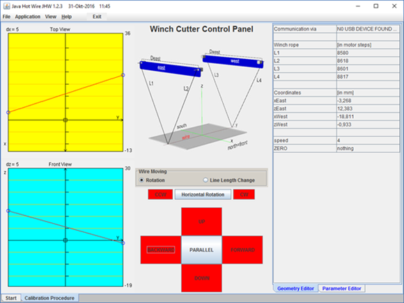
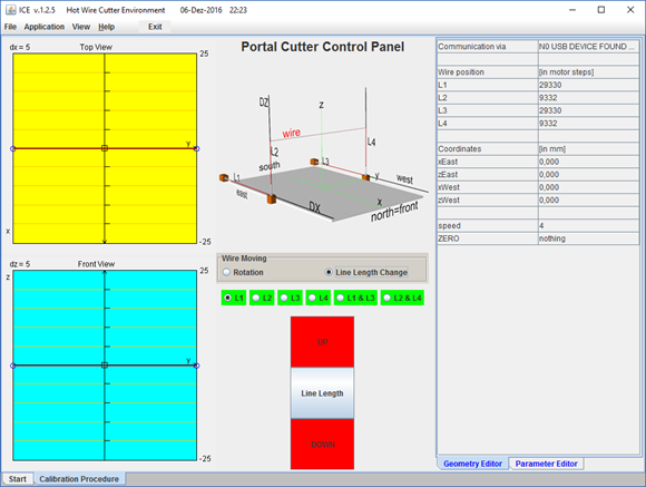
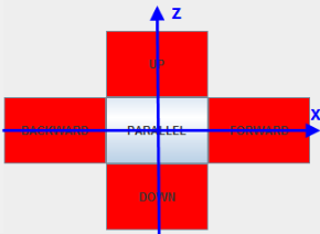
The cutting wire has four degrees of freedom (two parallel translations and 2 rotations). The new controller allows movement in these degrees of freedom.
1. Parallel shift in the z-axis: UP and DOWN
2. Parallel shift in the x-axis: BACKWARD and FOREWARD
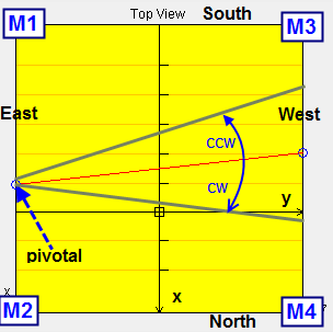
3. Rotation in the horizontal plane (xy plane) using this selector switch:
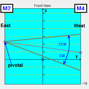
For practical reasons, the axis of rotation (in the picture marked with pivotal) is fixed on the east side. Why? It is always easier to look at the left suspension and to determine the necessary rotation, as to relate to another turning point, i.e. the center. This is particularly true for inexperienced users.

The rotations can take place clockwise (CW) or counterclockwise (CCW). There are no more possibilities!
1. Rotation in the vertical plane (yz plane) using this selector switch:
These complex movements (all four steppers work) are set by default. For whom these possibilities are not sufficient or do not like complex movements, can use the rope of his choice (check the box) and shorten (UP) or extend (DOWN) it, by clicking on .

The following applies to all movements: as long as the corresponding button is pressed with the mouse's cursor, as long as there is a movement. This behavior corresponds to the "dual rate" of RC remote controls. An exponential behavior is not implemented (I could not recognize its value so far). The speed level speed=6 is preset, but it can be changed according to your own ideas in the speed box where larger values correspond to slower speeds. Of course, single impulses can be generated by short clicks.

Movement and position of the wire can be controlled in the two schematic representations Topview and FrontView.

For all movements applies the following: the current parameters (properties of the system, namely (L₁, L₂, L₃, L₄, (x_E, z_E), (x_W, z_W)) )) appear right in the "property editor" (PE), all displayed in millimeters. If you don´t want to click, you can directly change the rope lengths in the PE (that is why it is called also an "editor").

The parameters of the system, which will be read out with the start of the program ICE from the geometry file hotwireGeometryData.prof define possible movements, and particularly their accuracy. The machine does not know the actual rope lengths, because there are no sensors for this. Similarly, there is no feedback on the location of the cutting wire to the computer and thus to the program ICE. All displayed coordinates refer to the geometrical data of the system but have nothing to do with the actual situation. Any changes in position are always of relative nature, i.e. relate to the current situation.

Geometry data, which represent the basic settings, and displayed parameters can be brought to cover only by an iterative adjustment and for this purpose the menu item ZERO is used (a kind of "zeroing" let's say). The current values are overwritten by the geometrical data of the system with "save" (left image below). In case of strong adjustment of the machine this is a useful approach. After several repetitions of this process you have achieved a perfect starting point for your cutting machine after a while (if you're carefully). Actual location and geometry data match - that's the point of calibration!

The cutting bow should be placed before powering down the system in a defined rest position. The best parking position is the central location. A careful parking usually eliminates most of the calibration work.

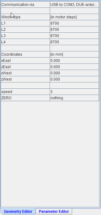
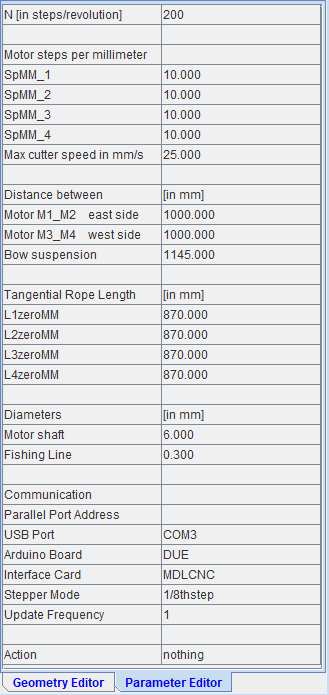
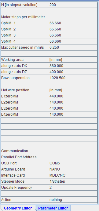
Using the parameter editor (right pictures) all relevant parameters of the cutter can be directly and comfortably changed. The same applies for the communication. Because there are no plausibility checks (it would be again a considerable effort to program them) you must be careful when choosing the input. For example, it makes no sense to enter together parallel port and USB. You can only use one or the other in a meaningful way. With Action = {nothing, save} you select whether the values you see in the editor should be saved or not. If you choose save ICE is automatically terminated. You must restart ICE again and only now your changed values are active.

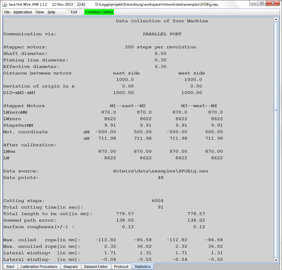
About menu "View", you can activate the card "Statistics", which contains all the interesting and uninteresting data on your machine and the cutting process that will assist in the control and optimization of machine parameters.
Graphical representation of data

The graphics you see in the tab "diagram" is based on the current data of the geometric figures. If you don't like the focus and therefore the size or location of the represented figure shown on the screen, you can easily change this at any time. All you need is a 3-button mouse. But if you don't have that, you cannot participate in the following procedure:

At first place the cursor into the area that attracts your interest mostly. Then scroll with the mouse wheel until the figure is tiny (zoom out). Then place the cursor into the figure and now scroll in the opposite direction (zoom in) until you are satisfied with the size of the figure. In each case, the area with the focus appears centered on the monitor. You can adjust the magnification that you prefer by sliding. You will know this procedure from CAD programs or also CorelDRAW which there is one of the standards.

If you want to enlarge an image area, you can achieve this by holding the left mouse button and moving to the right. The area to be crossed is highlighted in blue. If you have lost the image through diligent scrolling or you want to get back after any changes to the initial state, you move the mouse with pressed left button just to the left. The same is achieved by pressing the 'Reset' button.

Clicking with the right mouse button on the chart area leads to the menu items "Zoom In-Out". At this point axes can be zoomed independently of each other. With the menu item Autojustage you achieve a maximization of the graphics on the entire image size, however the common scale of the axes is lost here.

There are many equivalent actions that lead to one and the same representation. On the other hand infinitely many representations can be found which are all based on the same dataset and make no changes in the dataset! All these representations have no effect on the cutting data, however, changes in the data (see below) have an effect.

The representation options described are available in all graphics. During the cutting process you should refrain from such actions unless your graphics system is one of the faster, otherwise you will disturb the time regime of the computer.

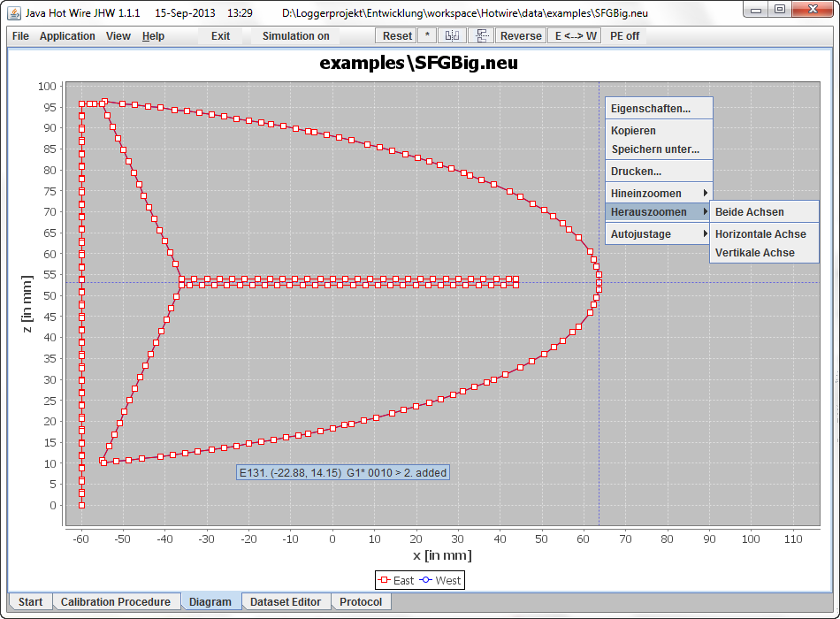
In the graph, two curves are drawn simultaneously, primarily the curve of the West-suspension (blue) and then that of the East-suspension of the East (red). If you see only a red line this means that the cutting bow moves parallel to the axes (but not for conical figures!).

If you move the cursor on a data point a tooltip appears with the following information:
{Number of data point (non zero-based), E/W, (x, z), point attributes}
When clicking with the left mouse button on a data point a crosshair with the coordinate values appears and you can evaluate the location of the data points relative to the other.

A click with the right mouse button on the chart area provides a menu to modify all chart parameters, i.e. you can color the chart here as it most closely matches your sense of beauty. You can also print out the chart using the print menu etc.

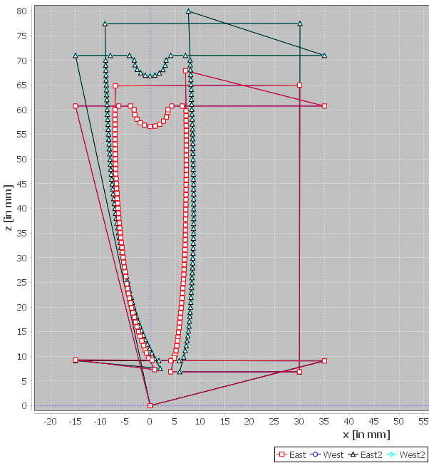
ICE offers the possibility to compare two data sets graphically. You enable the comparison by setting a check mark in the View -> Compare Dataset menu item. You are then prompted to load a second record. Only the formats *.how and *.dat are allowed. To close the comparison, remove the check mark in the View -> Compare Dataset menu item.

Data manipulation

Structure of the Dataset

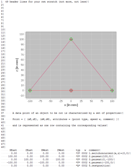
The dataset consists of a header and subsequent data points. The header includes 49 rows. Here you can be active as a writer and write what and as much as one likes, but it must be 49 lines in the end! The numbers 1-48 in the example below have no deeper significance - I did it to emphasize the necessary 49 lines.

The header is followed by the data points and each must be written in one line. A data point of an object to be cut is characterized by a set of properties with the following structure:

Point = { (x_E,z_E), (x_W,z_W), attributes = {type, speed w, comment} }

Example: 100.0 10.0 110.0 15.0 *P* 0003 2. pause at ((100,10);(110,15))

Interpretation:
From the current position the respective ends of the cutting wire are moved to the points East=(x_E,z_E)=(100,10) and West=(x_W,z_W)=(110,15)respectively, with the velocity w=3. In the points reached the action of type=*P* (i.e. pause) is performed. With comment="2. pause at ((100,10);(110,15))" this data point is annotated i.e. comment is a simple string type.

All coordinates are decimal numbers and represented as usual in computer science, by floating point numbers with a decimal point (e.g. "3.14". Commas (as common in German) can continue to be used. But ICE converts and saves this using the common international format, i.e. ICE is still compatible with the data files from Hans Seybold.

The data points can be separated by blank lines, which should contain no other characters. In this way, you can structure your dataset visually using newlines.

Datasets are always checked for identical successive data points and if necessary eliminated. For ICE it does not matter whether identical data points are included. But this is not valid for the cutting result. In the case of data doubling the wire stays twice as long and you get miniature grooves and no smooth surface. You will receive a notice on the "Protocol" with the message to save the dataset again.

Cutting process:
The coordinate point ( (0,0);(0,0) ) must be included in the dataset as first item. (0,0) is the wire's position after calibration. It moves to the first point of the dataset with w=2 and type=*A*. If no zero (0,0) exists, it will be inserted as 1-st point in the record temporarily, but removed after cutting.

Operations on the dataset

The menu bar contains several icons that allow basic operations on the dataset:

	With this icon the data points are (not) shown
	With this icon you can mirror the dataset at the ZY plane
	With this icon you can mirror the dataset at the XY plane (except points of the type "A" or "C")
	With this icon you can reverse the direction of cutting, i.e. the pass through the points {1, 2, 3 ... N} is done in reverse order, i.e., {N, (N-1), (N-2), ... 1}.
	With this icon you exchange East and West (for example to create a left and right wing)
	Restores the original dataset from which you started
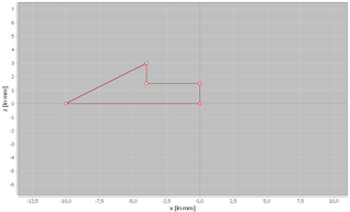
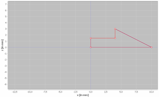
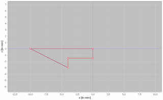
	Editor-Tableau

In the pictures you can see how the reflection works.

If you don't like the location of your geometric figure in space or you don't like a few points you can use a built-in editor to make changes to your data base. If you click on the button , the editor will appear with the two tabs Tools and Point.

Tools-Editor

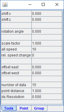
With this editor you can make translations and rotations of geometric objects. Together with the above reflection this will allow to reach all locations in space.

shift x [in mm]	implements a shift in the figure by the shift vector (x,z)
shift z [in mm]	except the points of the type "A" or "C"
rot α [in Grad]	causes rotation with the angle α around the centroid of the figure
scale factor f	causes a scaling of the figure by factor f, i.e. the point (x,z) transforms in (fx,fz)

In general, a geometric figure is represented by points, which generally have no constant point distances (constant point density). In the cutting process required points are determined iteratively by linear interpolation, which can cause errors especially when large distances have to be covered. To avoid such error conditions a constant point density is of advantage. This can be achieved by typing the desired distance for "point distance" with a default setting of 3 mm grid spacing. The points inserted by linear interpolation are always of the type "G1*" and get as comment the value ">new data". The speed is in each case taken from the last data point.

To change the speed of all data points (2 <= speed <= 32) you can do this with "all speed", whereat points of type A, S, D and C remain unchanged. With "rel. speed change" all speeds can be reduced or increased by the given value relSpeed in the range of -3 < relSpeed < 3 whereby points with speeds < 6 as well as of data typs A, S, E and C remain unchanged. Using this possibility a fine tuning of the thickness of the burned-in track can be performed.

In the pictures you see the action of these operations (left: rotation, right: scaling).

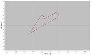
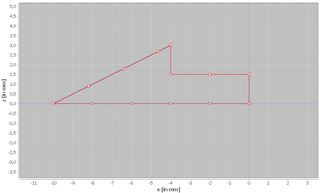
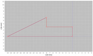
Using the option "offset" a new kerf can be generated or an existing one can be shifted for the east and independently for the west direction. When you do shell you need to pick a thickness value - it will be the shell thickness. Offset can be finicky - any little ripples in your geometrical object become magnified as offset tires to do a constant-distance offset away from the existing surface - the larger distance that you use tends to magnify any bumps and ripples in the object and if this causes the surface to bunch up together or cross over itself in any way, the shell will fail. So it is not unusual that you may need to shell with smaller values unless and this is a good idea you remove some tight bends or ripples in your object.

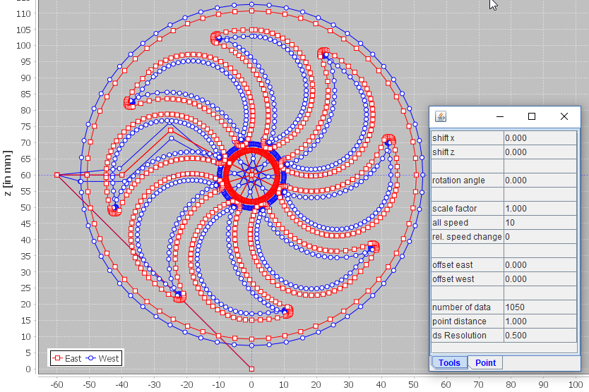
Concerning the input, in any case, all decimal numbers must be entered as usual in computer science, with a decimal point (e.g. 3.14)! After the change you have to click into another field to signal the editor that you have finished entering!!

Point-Editor

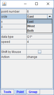
If you click on the tab "Point" you are inside the Point-Editor. It allows you to

- change
- delete
- add
- reorder
- cut (cutToEnd, deleteToEnd) points.

All values of a data point are accessible through the editor. If you move the mouse pointer over the data points the corresponding data values appear in an editor - Tableau immediately. By default the (x,z) - values of the East side of the cutting bow appear. The West coordinates can be reached when you double click the "Value"-cell from item "side". In a falling down menu (see right picture) you can select the side you want to see. The setting of "Both" shows always the values of the East side. If East and West sides should receive the same coordinates, set previously "Both" and then change the coordinates!

By clicking with the left mouse button on a chart point, a crosshair appears with the (x,z) values of the target point. Release the mouse button, a crosshair will remain on the nearest available data point. In this way, the points can be simply measured.

How does the Editor work?

Move the cursor to the point of your interest. The tooltip shows the point number which appears automatically in the editor or enter a different point number by hand. Immediately all properties associated with the point appear in the editor to which you may now have access and which you can change until they meet your expectations.

If you activate in the field Shift by Mouse the control box by double click, you can drag a point by mouse. The left mouse button moves east and west points in the same way, the right one influences the points individually. If a pop-up menu appears it can be removed by ESC without disturbing the image. As long as this mouse editor is active, the graph can not be zoomed. Deactivation can be reached again by double clicking Shift by Mouse.

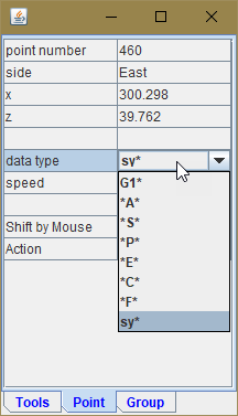
With the property "type" you can determine what should happen when such a point is reached during the cutting process. Currently, the following control characters are realized which can be addressed by double clicking on the "Value" field:

A		'Arrival' - from the offset point to the start point (high speed is possible)
G1*		Work area, where the cut is done (low speed for the cut)
C		'return' - to the offset point (high speed is possible)
S		'Stop' - i.e. cutting bow waits here; the comment in the dataset is displayed
P		'Pause' - i.e. the cutting bow waits, e.g. to set up the styroblock
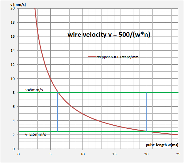
E		'Stop' - the cutting box stops here, the current must be switched off
F		'Fixed point' - which is not shifted during displacement along the z-axis.
sy*		'Point for synchronization' - used for tapered cutting

The property "speed" determines the velocity of the cutting bow. More specifically, this parameter is the time interval intended for a motor pulse in milliseconds, i.e. the smaller the value, the higher the cutting speed. Typical values are speed=2 for arrivals and departures as well as speed=15...20 for normal cutting speed. This information should be understood as reference speeds. Actual speeds depend on the cutting current, wire thickness, quality of the wire, material etc. and need to be determined experimentally.

If you want to cut for whatever reasons, with a horizontal velocity v_x[in mm/sec] the corresponding speed can be estimated using the simple relationship speed_x=27/v_x.You should remember here that the vertical velocity is always about 1.5 times larger according to the construction, so you have to decide for an average speed.

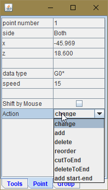
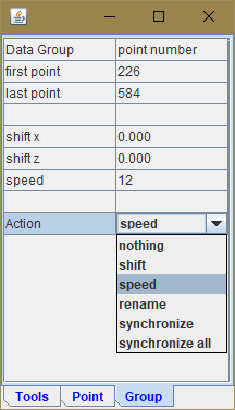
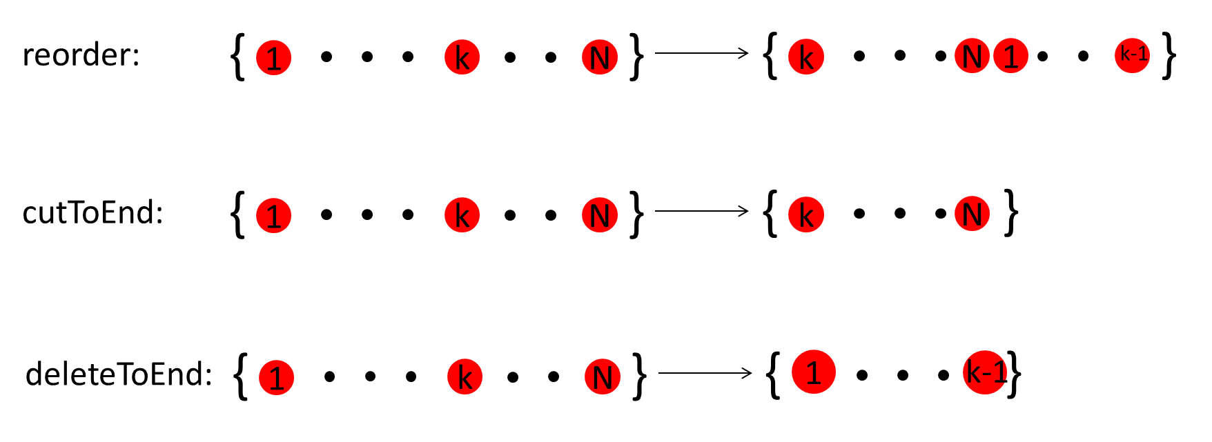
If you want to delete the point, you can do this by double clicking on the "change" field. This results in a Fall Down Menu (see right figure) with the values {change, delete, create, reorder, cutToEnd, deleteToEnd}. Selecting "delete" will delete the point, with "create" it creates a point. With "reorder" you can rearrange your data series beginning at the position k, i.e. from the set {1...k...N} the set {k...N|1...k-1} is created which is again numbered after the rearrangement from 1 to N. The value of k must be adjusted under "point number" before the rearrangement has been started. Thus, you have the ability to define the new starting point k in the cutting process.

Using the action cutToEnd all points beginning with number k up to the end can be cut out and on the other side with deleteToEnd removed. The pictorial representation summarizes these actions once again.

Dataset Editor

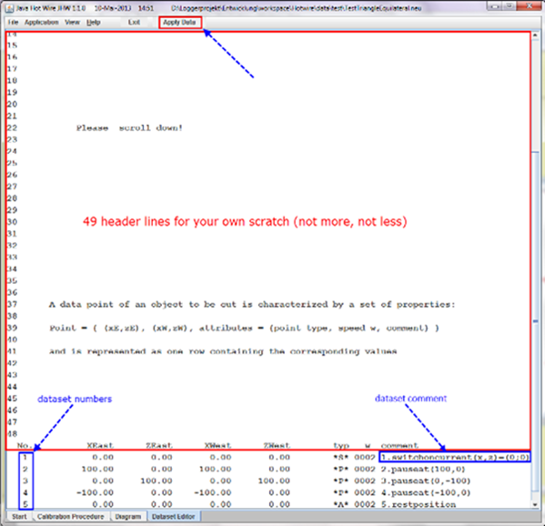
Clicking on "View → Dataset Editor" opens a full-fledged editor that allows editing the entire dataset. You may do everything, but the file structure and the structure of one record (a row) have to remain unchanged. The header line must be in the first place! You can delete records, regroup or add. The record numbers are not of your concern, they only serve as easy orientation and have otherwise nothing to imply, but they must be present! - Otherwise you will generate an error message.

Every dataset line has at its end a comment area comment beginning with the speed w. Here you can write whatever you want otherwise let it free.

With "Apply Data" the data shown in editor are taken over and graphically represented in the tab "Diagram". Thus the data can be adjusted or rebuild by alternately switching the two tabs "Dataset Editor" and "Diagram" interactively in a direct way very comfortable corresponding to your own ideas.

In principle the current dataset is graphically displayed in "Diagram" and mapped in "Dataset Editor" so you always have a precise control over all made manipulations.

Should your current graphics and/or changes no longer appeal to you click on the "Reset"-icon and immediately the original dataset will be restored.

Data structure beginning with version 1.2.0:

The old data structure is given here for the sake of completeness. Such data files can only be read. Basically, the new data structure is used for saving beginning with version 1.2.0.

Simulator

A 2D-simulator which passes through the cutting record simulating the cut can be started with the icon "Simulation". It can be operated via player controls known to everyone in the modes {"Stop", "Single Step", "Continue/Start"}.East and West suspension of the cutting bow are displayed simultaneously, but in the drawing sequence West - East. If the two paths agree with each other only the East curve (red) can be seen. You can repeat the simulation with the player icon "Start" and then the last set of simulation speed is used.

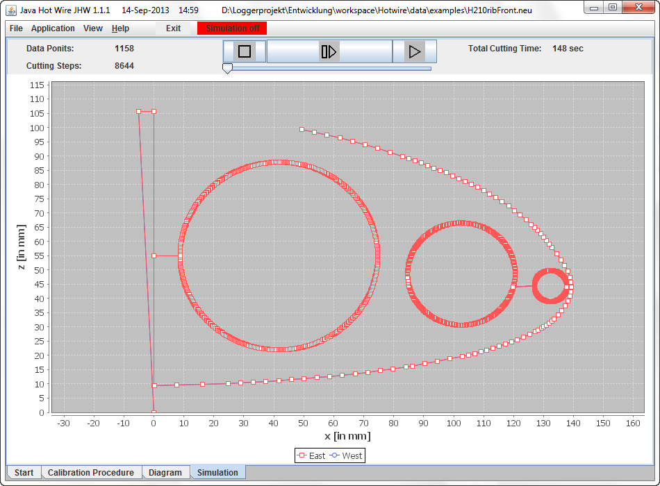
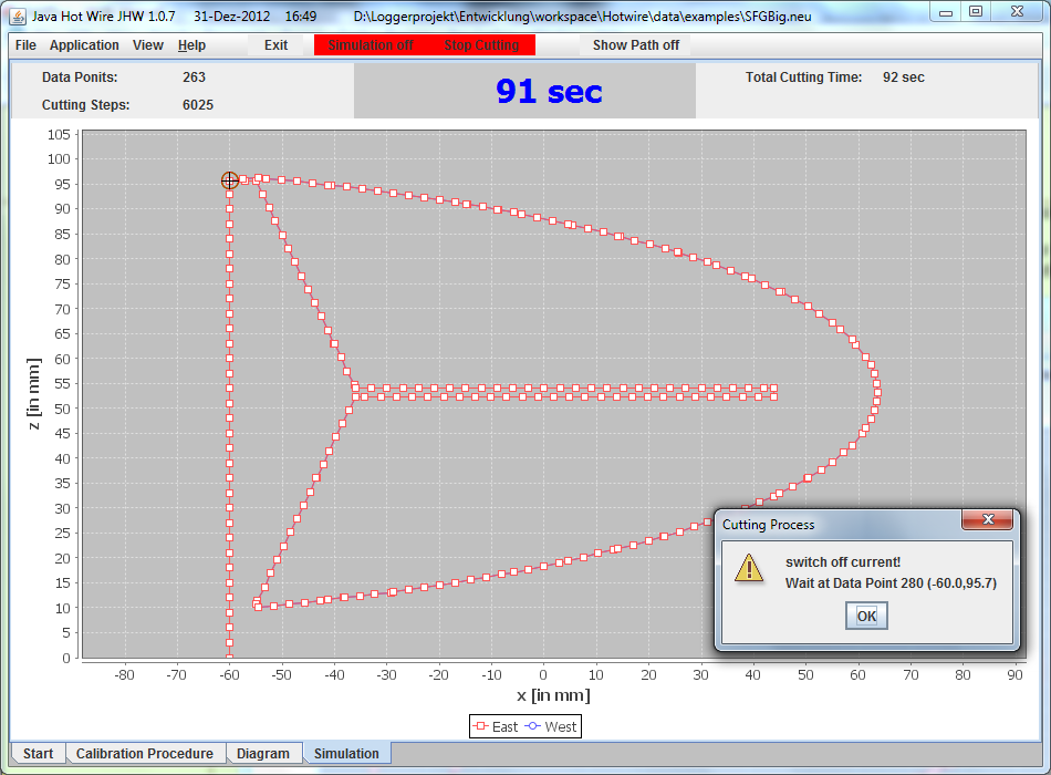
After a successful simulation the new icon "Start Cutting" appears. With this icon the actual cutting operation can be started. With the also newly added switcher "Show Path on" / "Show Path off" the current cutting position can be traced during the cutting process simultaneously on the screen. To be able to afford this luxury, you should have however a powerful computer (better graphics card), otherwise the cutting process is disturbed!

According to the type property of the points the cutting operation pauses with an information message. The progress can be continued with "ENTER". With the help of the "Slider" you can set the simulation speed. The simulation can be repeated as often as desired.

The icon "Stop" serves to stop the cutting process (in order to give the cutting block a new location for example), with "Continue" you continue or clicking again to "Stop" cancels completely the cutting process. Then the cutting bow is returned to its starting position.

3D-Simulation

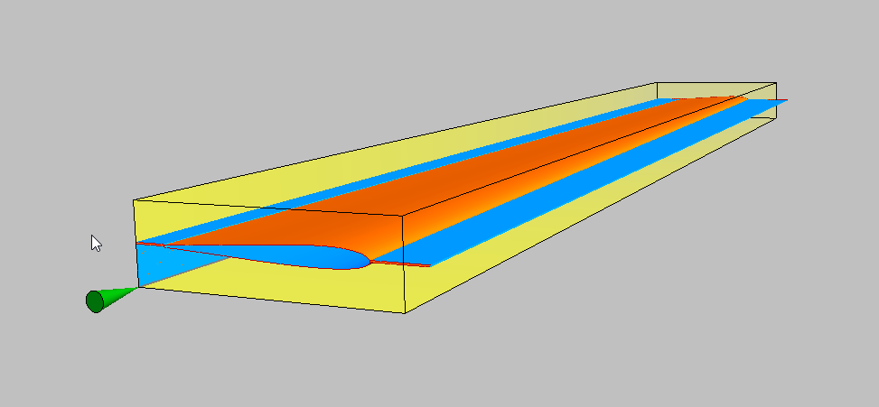
If you want to have a special pleasure, you can look at your data in a 3D-simulator. Rather new insights are not obtained, but it is rather nice:
Application
Data generation with ICE

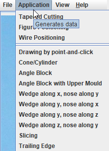
Cutting data of pre-built standard tasks can be generated via the "Application" menu item. In all cases, clicking on Apply Data the data is copied to the editor, which can then be edited via "View -> Dataset Editor" .

Menu item Tapered Cutting

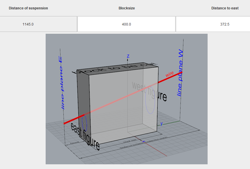
In order to produce conical cuts, the cutting data of the east and west figures (which are to be produced on the east and west sides of the block) must be transformed to the respective bow suspension.

Menu item Figure Positioning

Here you have full access to the geometric figure you want to cut.

Menu item Wire Positioning

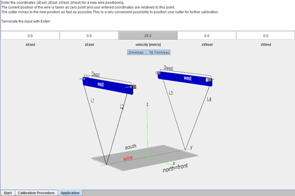
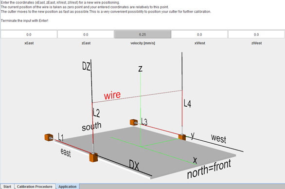
Enter the coordinates (xEast, zEast) and (xWest, zWest) to which you want to move the cutting wire. The current wire position is assumed to be a zero point, and the coordinates entered are relative to these. The cutter moves towards this position at full speed. This is a convenient way to position the wire for further calibration.

Menu item Drawing by point-and-click

This offers the possibility to create records by
1. Retracing of a master illustration (left)
2. Free-hand drawing (right)
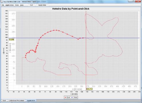
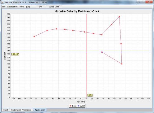
In both cases, the drawing is done by mouse clicks. The points are then connected by a continuous curve in order to guide the eye better. The drawing pattern (graphics file formats of .png, .gif, .jpg) can be loaded via Load. It does not matter which format you use or in other words, there is no format that one would necessarily prefer. If no picture is required you can immediately start with the drawing via Application --> Drawing by point-and-click.

If you are happy with your art than by clicking on Apply Data the data record is transferred and displayed on the tab Diagram and can be as usual, if necessary, further manipulated and finally stored. Keep in mind that this procedure using a master image does not provide true to scale representations (this has principal reasons)! So you have to make the desired scale yourselves but this is very simple by using the scale factor-function in the tool editor Tool-Editor.

Menu item Cone/Cylinder

Using this application which allows to build aircraft fuselages, data for a cone or cylinder (both of circular and elliptical shaped) can be created. On the tab "Application" an input form appears where you can enter your parameters.

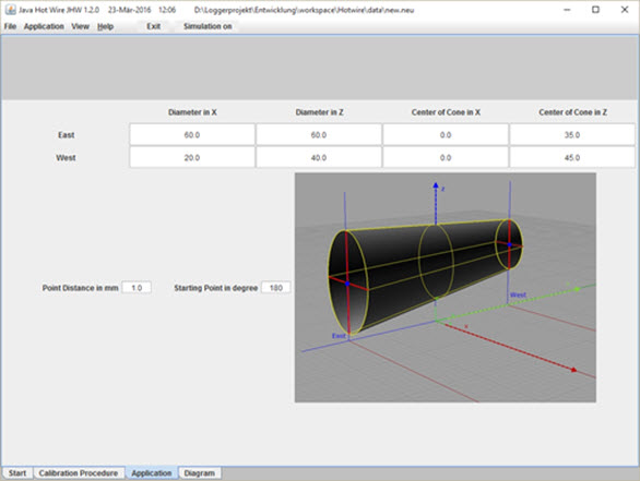
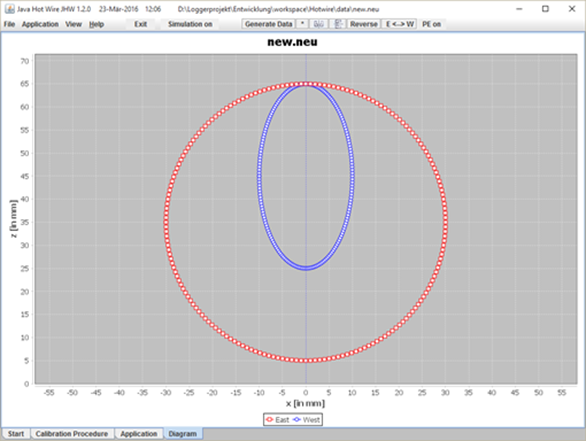
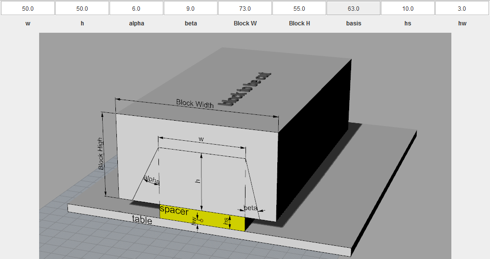
Menu item Angle Block

Using this application, any angle blocks can be created e.g. a grainding block. On the tab "Application" an input form appears where you can enter your parameters.

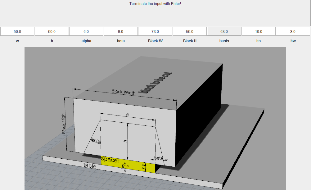
Menu item Angle Block with Upper Mould

Using this application, any angle blocks can be created e.g. a grainding block. On the tab "Application" an input form appears where you can enter your parameters.

Menu item Wedge

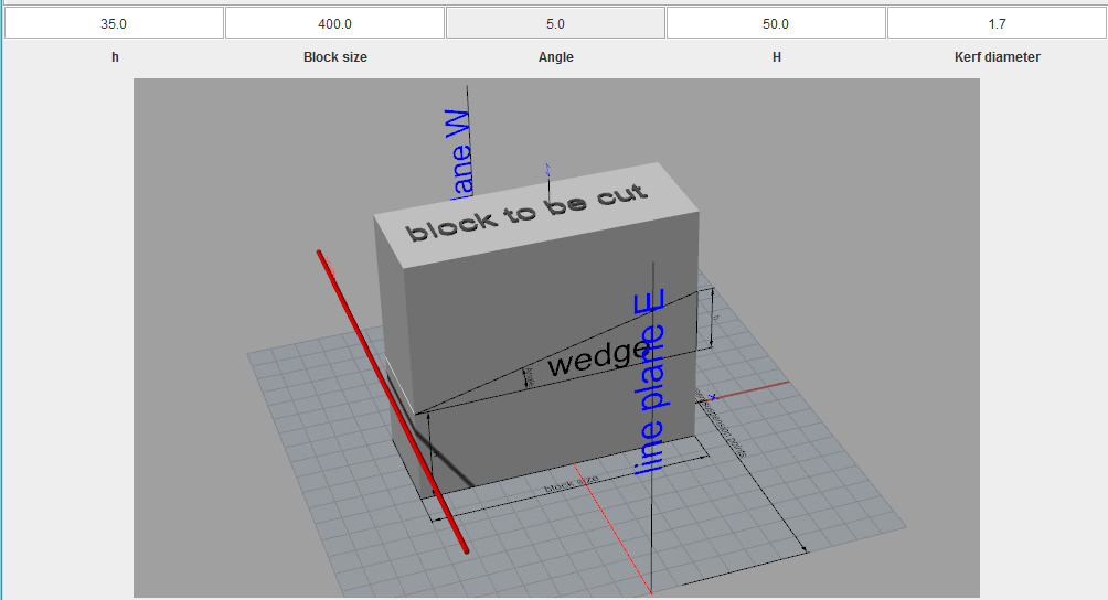
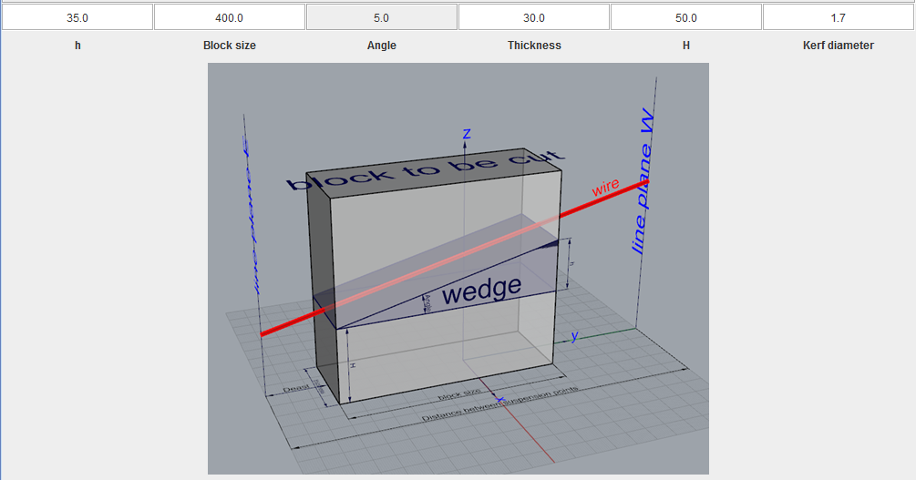
Using this application, any wedges can be generated. An input mask appears in which you can enter your parameters. The wedge can be produced in two different ways: The wedge is cut in the x-direction, i.e., from south to north with a parallel wire. In the second variant, the wedge lies parallel to the y-direction and is cut with an inclined wire.

Menu item Trailing Edge

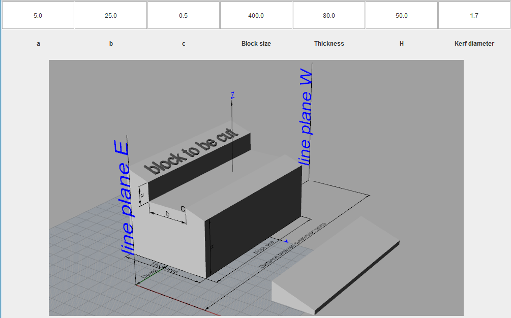
Using this application, grainding templates for trailing edges can be created. On the tab "Application" an input form appears where you can enter your parameters.

Examples

Form to laminate

Help

In the directory help or myhelp you can view your own files in the format htm, html oder txt. Use HTML if you want to include images:

                <html>
                <body>
                <img src="nicePicture.gif" alt="Help" title="So it's better!" />
                </body>
                </html>

Installation

Check in the DOS console using the statement java -version. The answer should be:

c:\Program Files (x86)\Java\jre\bin>java -version
java version "1.8.0_60"
Java(TM) SE Runtime Environment (build 1.8.0_60-b27)
Java HotSpot(TM) Client VM (build 25.60-b23, mixed mode)

Otherwise proceed as follows:
Download the file jre-8u60-windows-i586.exe or higher ( Download page 1 or Download page 2 or ...). This file contains everything needed to install the 32 - Bit - Java Runtime Environment(JRE), including the installer and character conversion classes and support for locales other than the US English locale. Please note in order to install the Java Runtime Environment and the libraries further below on Microsoft Windows 2000, XP, Vista, 7 , 8 or 10 you must have administrative permissions.

If you want to use the cutting module (menue Start Cutting after simulation) proceed as follows:

! You have to install jnpout32pkg.dll

i.e. the file jnpout32pkg.dll (if the link does not work you will find it in subdirectory lib) must be stored in the Windows Environment:

jnpout32pkg.dll

⇒

%WINDIR%/system32

If the cutting module does not work, please check your computer. May be, there is no Parallel-PORT at all! If so, sorry, I can nothing do for you unless you have extended your system by an Arduino board which uses USB.

ICE communicates with the serial Arduino device through the RXTX library available from http://www.jcontrol.org/download/rxtx_en.html (if the link does not work you will find it in subdirectory lib). RXTX consists of two parts: The Java extension library RXTXcomm.jar and the native serial driver to be integrated with the operating system. RXTX must be installed after having installed JRE.

RXTX Java serial controller RXTXcomm.jar	⇒	into the lib/ext folder of the 32-Bit-Java VM
RXTX native driver rxtxSerial.dll	⇒	into the bin folder of the 32-Bit-Java VM

Some hints concerning the accuracy of your cutting device you can find here.

ICE Directory Structure
Download the ZIP package and unpack it to your favorite location (USB stick, ...). ICE runs without any additional installation and won't store any settings outside the application directory. The program is distributed with the following directory structure. It is strongly recommended to retain this order. Ofcourse you can keep your data in an arbitrary directory but don't touch the hotwire-subdirectory.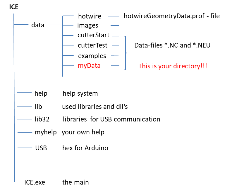

Licence

The program ICE is free software only for noncommercial use. It is distributed under the terms of the GNU Lesser General Public Licence (LGPL). ICE is distributed in the hope that it will be useful, but WITHOUT ANY WARRANTY; without even the implied warranty of MERCHANTABILITY or FITNESS FOR A PARTICULAR PURPOSE.

Tips

Before you start the cutting process itself an initialization is required. In principle, you can start from any point and set this point as a reference point. But this is not very useful. The zero position of the machine should be characterized by a high degree of symmetry, and there is only one position in question, namely the middle position, in which all four ropes have the same length. In any case, if you start the machine this should always be done from the central point location, i.e. x = 0 and z = (2-3) mm. This starting point found during the calibration process defines the origin. There is no other origin! This situation which is interpreted by the software as a (0, 0) minimizes systematic errors. The software takes into account the finite geometry of the system components. This only works when the machine starts exactly in such a manner as required by the software.

The Styropor, Styrodur or Depron (EPS, XPS Foam etc.) or block from which you want to cut out your subject should be if possible placed in the center of the cutting table that is symmetrically to x = 0. Always make sure that you cut from back to front: then for setting up the block you never have to grab across the hot wire! To achieve this you should prepend the record with two lines as well as two lines at the end. The first point of the dataset is also the first point, to which the cutter moves. Thus, one doesn't really need the "go to zero" statement in the dataset, because the machine is after calibration already in zero position. But if it is there, it will not hurt.
The wire is moved to the second point (x₀,z₀) and stops. Now you can unhurriedly prepare the foam block to be cut and start the cutting process by pressing ENTER. Finally the wire stops at the point (x_end,z_end). Here the cut foam can be removed from the machine before the wire returns with ENTER to the zero position.

0,0 0,0 0,0 0,0	A 0002 go to Zero position	Arrival at Zero Position
x0 z0 x0 z0	S 0002 stop to prepare the block	stop to prepare the block and switch on current
Dataset		This is the right place for your dataset!
xend zend xend zend	S 0002 stop to switch off	Stop to switch off current and to remove everything
0,0 0,0 0,0 0,0	C 0002 go to Zero position	Return to starting point

From the block the wire cuts out the geometric object. During cutting a physical quantity comes unexpectedly into play, against which my software can do nothing - the force of gravity. The half cut out core lowers due to its weight to the width of the combustion track causing deviations in the further progress of cutting. If you want accuracy you need to stabilize the core e.g. by inserting small wedges etc., in any case the software has nothing to do with such accuracy problems.

Often one is faced with a typical situation: For some reason you would like to put the block to be cut on a spacer of height H. The distance from the object to be cut - bottom edge of the block may be h.

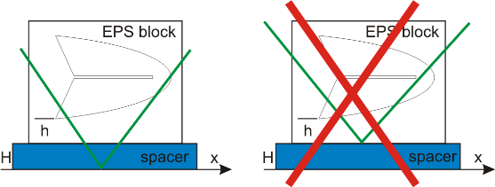
How to do: With the help of the program the object to be cut is shifted by the function "shift" by (x,z) = (x0, H + h) which is indeed very simple using the supplied function (see Tool-Editor).

A second option could be to produce manually (a new calibration) on a spacer of height H a new zero position, then put the block to be cut on the spacer and start cutting displays incorrect results because the coordinate transformations in the cutting space is not translation invariant, i.e. the zero point cannot be moved by transformation.

The tensioned wire is heated by an electrical current source which causes the wire to heat up. The heat energy that radiates off the wire melts the foam. Enough heat is generated by the wire that the foam will melt in front of the wire as it moves through the foam. The amount of power that runs through the wire and the speed that the wire travels is important. Set the power too low, and the wire will cut by contact. Increasing the amperage the amount of foam that is melted will be more excessive. Also with too much heat, the surface of the foam is distorted. Cut too fast or slow and you will either cut by contact or melt too much foam.

The kerf is the thickness of the foam melted by the Hot Wire. The slower the hot wire travels, the larger the kerf is. The hotter is the wire, the larger the kerf is. You can evaluate the kerf value with a cutting test, with your current speed and temperature values on the same material (there are just many different types of foam having all different properties..).

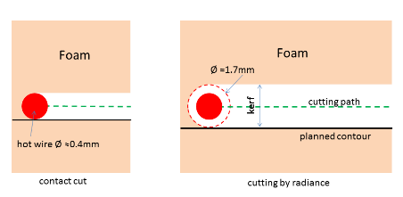
The special cutting wire Type 2001 Nickel-Chrome-Titanium copper coated can be used very favorably with a diameter of 0.4 mm (= 0.016") which poses absolutely no problem due to its unique characteristics: elongation at over 1,800 - 2,000 N/mm² tension @ 680°C ( =1,256° F) is less than 3%. The wire has a very good surface which during cutting does not tend to stick. The wire also seems to be very resistant to corrosion by chlorine which can be supported by cleaning immediately after cutting.

Cutting speed and cutting current:
The following cutting speeds and cutting currents have proven themselves with the standard cutting wire (Ø0.4mm) and can be viewed as a good guideline:

Density of foam [in kg/m³]	Cutting speed [in mm/sec]	w [in ms]	Cutting current [in A]
EPS 12 - 18	5 - 8		2.3 � 2.5
EPS 20 - 25	3 - 5		2.5 � 2.7
XPS 25 - 40	3 - 5		2.6 � 2.8
XPS 20mm(yellow)		16	2.6
XPS 20mm(yellow) as block(500mm)		16	2.8
Styrodur(green P3035CS) as block(500mm)		16	2.7
Rohacell IGF31 as block(500mm)		25	3.7
Depron 4mm		15	2.5

Cutter

If you want to use the program ICE to cut you have to make sure you can use the following rotation of the stepper motors (clockwise (CW) or counterclockwise (CCW)) standing and looking at the east side. This can always be done by reversing two motor contacts, no matter how the engines are mounted and is valid for both rope geometries.

to coil up to uncoil

Motor 1 and 3 CW CCW

Motor 2 and 4 CCW CW

If the cutting wire of your machine is guided via guide loop you must deactivate the RADIUS correction by setting the effective radius to zero in your geometry data, i.e. DS_effective=0 (see data management).

In this context, I have found a rope which can be considered a true super-rope and has proved itself excellently: diameter 0.3mm, material Coramid, extremely pre-stretched (Climax Protec red).

Stepper Controller
The ICE program has been developed at our foam cutter in the model club Rossendorf, which works on the basis of the MDLC CNC stepper controller board, a professional stepper motor driver for 4 universities-/bipolar stepper motors. It works after the constant current principle for optimum torque at higher speeds and is characterized by professional feature set. The card is designed to the build own hobby CNC machines. The board is comptible with many software solutions. This card uses as interface the popular parallel port, i.e. communication with the PC (i.e. ICE) must run on this. ICE generates the cutting information (clock c and direction d information) for each of the stepper motors M1, ..., M4 via the PC parallel port interface with the pin configuration shown here. The same pin assignment is also used by the MDLC board. If stepper controllers from other manufacturers have also a parallel port, there should be no problems to make an appropriate pin adjustment.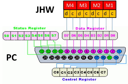

Parallel Port-Communication
The simplest way to rialize a communication between PC and stepper controller consists in connecting both via an ordinary printer cable.

But there are difficulties with modern computers, because you will hardly find a parallel port interface in them.

A low cost option is to get for a few euros an "EX-41001 1P PCI Parallel Card". It can be easily plugged into your PC provided a free PCI slot is available. In such a simple way you have shouted your PC with a parallel port.

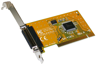
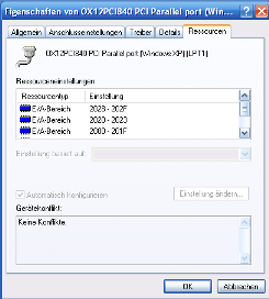
This EX-41001 PCI parallel adapter provides one SPP/EPP/ECP high performance port. It is designed for PC, thin client or server to provide instant LPT port expansion via the PCI-or PCI-X Bus. The card is fully Universal PCI Plug-and-Play compatible and there are no IRQ and I/O address configuration problems.

The so upgraded PCI parallel port has its address at 0x2028 and cannot be readjusted at the usually used standard address 378hex = 888dec. In order to reach the parallel port you have to modify the file "hotwireGeometryData.prof" by adding

PPportAddress 8232

as last line if your parallel port address should be 0x2028 (0x2028 = 8232dec) as in the above case and then everything works, so again in detail:

USB-Communication
Today's computers are equipped with USB interfaces in sufficient numbers. Consequently, you need a software solution that combines these two interfaces. ICE since version 1.1.6 can communicate with the PC via USB. The connection is made according to the following scheme. A microprocessor Board of type Arduino (NANO, UNO or DUE ) is interposed and is currently running with software version "HotwireV0.9UNO/DUE". Recently, the very new and high-performance 32bit-boards Teensy 3.2 - 3.6 can be used. Please do not forget to tell the system to which serial port the Arduino board is connected.

Has the USB communication benefits?

Yes, for sure. Not to mention that fact that modern computers mostly lacking of a parallel port. But these advantages come only into its own, when going from full step to half step or even better, to micro step mode, as long as step motors and control board allow this ability. Then the entire system runs very quietly and does not tend to oscillate. The cut quality can be improved massively.

Why is that?

There are at least two reasons. Generally stepper motors are said to be accurate. That's not so because they have a target deviation. Whenever the rotating field will jump one step or half-step, the rotor follows jumping - and oscillates around its new magnetic equilibrium point. In practice, depending on mass, inhomogeneity's in the magnetic field, friction and load, he will stop somewhere next to the theoretical target point.

The angular tolerance of a "normal" stepper is around +/- 5% from full step. A precision motor tends to approximately +/- 2 to 3%. Commonly used 5 € motors would amount to rather +/- 10%. A micro-step control allows to increase the fine positioning since a half-step control doubles and a 1/8th control generates an 8-fold number of steps. Therefore, it also requires twice or 8 time as much data. A 1/16th micro step already falls within the tolerance range mentioned above. Any higher micro step resolution of a "normal" stepper is simply a "nice to have", in other words, useless.

Stepper motors need equidistant clock pulses. When pulses vary within a few percent at an intended uniform movement of the motor, this means that the stepper is decelerating. If a clock pulse is generated too late, the stepper gets a negative acceleration. If the next cycle is again generated at the correct time, the motor will accelerate to continue its movement. But it should really perform no acceleration as it should move smoothly. The result is that the stepper vibrates. In addition, it consumes an unnecessary amount of kinetic energy and loses torque at the same time, as it has to spend a large part into permanent accelerations. The styro cutter represents an oscillatory system and strong vibrations are more or less generated. The cutting wire passes them on as visible groove structures in the cutting surface.

This problem usually occurs when you use the PC, for example, to transmit signals via parallel port (all our major operating systems are non-real-time capable). The problem can be reduced by minimizing the number of applications running on the PC simultaneously. A micro-step mode is excluded because this communication requires a greatly increased data transfer and is therefore much strained.

This problem can only be solved using a control board with a MC which generates highly accurate clock pulses for the stepper motors. Realizing this, the MC board must be supplied via USB with the data generated in ICE.

References

H. Seybold:	CNC-gesteuerte Heißdrahtschneidemaschine, Styroschneider nach Konzept Hans23
Video	A short introduction to ICE only in German but nevertheless...
Letmathe:	CNC-Technik
W. Stratmann:	BOcnc
S. Duranti:	Profili
Cutter elements:	CNC products
Fishing line:	Climax Protec
Cutting wire:	offer
Arduino:	Arduino DUE
Teensy:	Teensy

Topics about the environment

A short introduction into foam

Mathematical basics of an hot wire foam cutter

A short help for format conversion

Cutting data in the 3D-Simulator

USB communication

Tests und parameters to adjust the cutter

Creation of a mould to laminate

Synchronization of data for tapered cutting

Development

V1.4.2

2.05.21

-        Optimization of tapered cutting

-        Smaller Bug fixes

V1.4.1

25.06.20

-        Optional calibration with the key board

-        Smaller Bug fixes

V1.4.0

30.10.19

-        New functions for the group editor

-        Extension of the tool for synchronization for tapered cutting

-        Tutorial for the synchronization tool

-        Extension of the merge function

-        New applications

-        Improvement of the group editor for data points

-        Improvement of the program handling

-        Smaller Bug fixes

V1.3.9

12.2.19

-        Data converter for the import of Winghelper files of .ngc format
-        Improvement of the group-editor for data points

-        Smaller Bug fixes

V1.3.8

25.12.18

-        Improvement of the program handling

-        Smaller Bug fixes

V1.3.7

15.03.18

-        Goup Editor for data points

-        Smaller Bug fixes

V1.3.6

15.02.18

-        Editor for synchronization

-        Attention: change of the data set!

-        Smaller Bug fixes

V1.3.5

26.01.18

-        New cutting engine

-        Revision of the manual

-        Smaller Bug fixes

V1.3.4

12.01.18

-        Improvement of the synchronization between east/west figures for the tapered cut

-        Discussions with Winghelper lead to an ICE export function of .how files in Winghelper

-        Smaller Bug fixes

V1.3.3

5.01.18

-        Merge function: east und west figures from two different files

-        Smaller Bug fixes

V1.3.2

15.12.17

-        Extension of the file converter

-        Smaller Bug fixes

V1.3.1

11.12.17

-        Improvement of the cutting process control

-        Smaller Bug fixes

V1.3.0

25.10.17

-        USB with 32bit-boards Teensy 3.2-3.6

-        New formulation of the Arduino firm ware V1.11

-        Smaller Bug fixes

V1.2.9

2.04.17

-        Improvement of the USB-communication

-        Modification of the USB-communication protocol

-        Optimization of the Arduino Software V1.08

-        Smaller Bug fixes

V1.2.8

1.03.17

-        Heating control

-        Optimization of the Arduino Software V1.07

-        Smaller Bug fixes

V1.2.7

1.02.17

-        Optimization of load/save

-        Data files can be saved in G-code

-        Reformulation of the G-code converter

-        Reformulation of the dat converter

-        Converter for GMFC files

-        Connection to the 3D-Simulator devSimCnc Foam from devcad/Profili

-        Smaller Bug fixes

V1.2.6

11.01.17

-        Extension of the USB-communication protocol

-        Optimization of the Arduino Software V1.00

-        Smaller Bug fixes

V1.2.5

1.12.16

-        Menu item Data Compare: two data files can be compared graphically

-        Optimization of the simulation

-        Smaller Bug fixes

V1.2.4

1.11.16

-        Extension of the application spectrum of ICE

-        Smaller Bug fixes

V1.2.3

1.09.16

-        Application: production of an angle block with upper mould

-        Fast manual cutter positioning

-        Extension of the calibration

-        DAT - files can now be processed. This format allows you to import airfoils.

-        Smaller Bug fixes

V1.2.2

9.08.16

-        Data storage in format *.how with 3 decimal places

-        Improvement of the NC-converter to import NC-data

-        Smaller Bug fixes

V1.2.1

4.05.16

-        East-west-positioning and rotation of the geometric figure

-        Transformation to bow suspension to produce conical cuts

-        Application: production of an angle block

-        Application: production of a wedge

-        Application: grainding templates for the trailing edge

-        Improvement of the Help System

-        Improvement of the NC-converter to import NC-data

-        Smaller Bug fixes

V1.2.0

5.12.15

-        New data structure *.how, but the old one can be read

-        New file information system

-        Revision of the USB communication

-        Half, 1/4th and micro step mode can be configured in ICE

-        Extension of the Arduino Software V0.9

-        Improvement of the Help System

-        Smaller Bug fixes

V1.1.9

16.10.15

-        Revision of the USB communication

-        Different CNC controller types and Arduino Boards can be configured in ICE

-        Extension of the Arduino Software V0.2

-        New Hotwire Parameter Editor

-        Smaller Bug fixes

V1.1.8

11.12.14

-        The parallel port address is now adjustable.

-        Some tips

-        Smaller Bug fixes

V1.1.7

10.09.14

-        USB with Arduino NANO, UNO, DUE Board

-        Smaller Bug fixes

V1.1.6

01.05.14

-        Communication with the stepper controller via USB

-        Microprocessor Arduino DUE Board - Programming

-        Smaller Bug fixes

V1.1.5

24.12.13

-        Optmization of the stepper controller

-        Offset-East und West independently from each other. So you can generate und change kerfs.

-        Cutting process is automatically done with a constant point density of 1ppmm performed by linear interpolation.

-        Smaller Bug fixes

V1.1.4

20.11.13

-        Improvement of the accuracy by taking into account non-linear effects due to finite geometry.

-        Cutting process is automatically done with a constant point density of 1ppmm performed by linear interpolation.

-        Smaller Bug fixes

V1.1.3

11.11.13

-        Optimization of the trajetory tracking. Why only now? Mathematically extremely time-consuming...

-        Smaller Bug fixes

V1.1.2

11.10.13

-        A modul for statistics summerizes all machine parameters used and allows a control of the cutting process.

-        Smaller Bug fixes

V1.1.1

11.09.13

-        Improvement of the NC-converter to import NC-data

-        The Tools-editor allows a relative change of the velocity of cutting by a given value.

-        Im Tool-Editor können Schneidegeschwindigkeiten relativ geändert werden

-        Smaller Bug fixes

V1.1.0

10.06.13

-        New cutting engine

-        Representation of all flouting point numbers by "." where&xnbsp; comma during input is still tolerated.

-        The dataset can contain blank lines; &xnbsp;elimination of doubling of data points

-        Application Cone/Cylinder was revised

-        Geometry data file for adjustment of Hotwireprofils (hotwireGeometryData.prof) is changed!

-        Smaller Bug fixes

V1.0.9

31.04.13

-        New calibration modul

-        Smaller Bug fixes

V1.0.8

25.02.13

-        Internal optimization (barely visible from the outside)

-        Smaller bugs

V1.0.7

31.12.12

-        Retracing of a master illustration by point-and-click

-        Free-hand drawing

V1.0.6

28.10.12

-        Extension of the Data Editor functionality

-        Extension of the Point Editor by a Mouse Editor

V1.0.4

18.12.11

-        Geometry data file for adjustment of Hotwireprofils (hotwireGeometryData.prof) is changed!

V1.0.3

2.11.11

-        cutting process runs in its own thread

-        cutting speed can be adjusted freely

-        Cutting process is automatically done with a constant point density of 3ppmm performed by linear interpolation.

-        New function added: "all speed" in the Tools editor, so you can change the cutting speeds of all data points.

V1.0.0

26.8.11

-        published as full version

-        Data Editor

V0.9.6

24.8.11

-        Data saving in format *.neu with 2 decimal places, unlike to H. Seybold.!

V0.9.5

3.3.11

-        cutting process was formulated as Event-controlled process

-        auto scaling revised

V0.9.3

19.2.11

-        Fixed bug when saving

-        G-code(NC-data) can now be processed

-        Auto-scaling of the jfreechart library is incorrect, replaced by self-made module

V0.9.2

15.2.11

-        publication

V0.9.1

3.11.10

-        taking into account the finite geometry (diameter of motor shaft, rope)

V0.9.0

4.10.10

-        Start of programming

	to coil up	to uncoil
Motor 1 and 3	CW	CCW
Motor 2 and 4	CCW	CW

ICE Manual

Structure of the Dataset

Operations on the dataset

Tools-Editor

Point-Editor

! You have to install jnpout32pkg.dll